Bii o ṣe le ṣe afiwe awọn ọwọn meji ni Excel ati yọ awọn ẹda-iwe kuro (aami, awọ, gbe)

This article will take you about 10 minutes to read. In the next 5 minutes, you can easily compare two columns in Excel and find out if there are duplicates in them, delete them or highlight them in color. So, the time has come!

Excel is a very powerful and really cool application for creating and processing large amounts of data. If you have several workbooks with data (or just one huge table), then you probably want to compare 2 columns, find duplicate values, and then do something with them, for example, delete, highlight or clear the contents . Columns can be in the same table, be adjacent or not adjacent, may be located on 2 different sheets or even in different books.

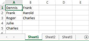
Imagine we have 2 columns with people’s names – 5 names per column A and 3 names in a column B. You need to compare the names in these two columns and find duplicates. As you understand, this is fictitious data, taken solely for example. In real tables, we are dealing with thousands or even tens of thousands of records.

Aṣayan A: both columns are on the same sheet. For example, a column A ati ọwọn B.

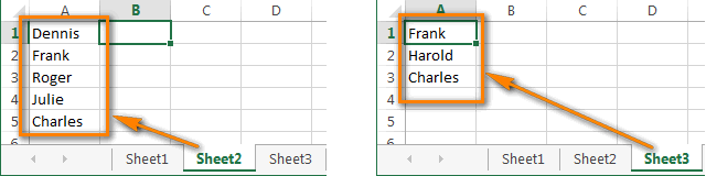
Aṣayan B: The columns are on different sheets. For example, a column A lori dì Iwe 2 ati ọwọn A lori dì Iwe 3.

Excel 2013, 2010 and 2007 have a built-in tool Yọ Awọn ẹda-iwe kuro (Remove Duplicates) but it is powerless in this situation as it cannot compare data in 2 columns. Moreover, it can only remove duplicates. There are no other options such as highlighting or changing colors. And point!

Next, I will show you the possible ways to compare two columns in Excel, which will allow you to find and remove duplicate records.

• Compare 2 columns and look for duplicates using formulas
  
  • Option A: both columns are on the same sheet
  • Option B: The columns are on different sheets or in different workbooks
• Processing of found duplicates
  
  • Show only duplicate rows in column A
  • Change color or highlight found duplicates
  • Remove duplicates from first column

Compare 2 columns in Excel and find duplicate entries using formulas

Option A: both columns are on the same sheet

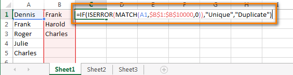
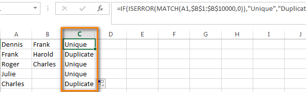
1. In the first empty cell (in our example, this is cell C1), we write the following formula:

   =IF(ISERROR(MATCH(A1,$B$1:$B$10000,0)),"Unique","Duplicate")

   =ЕСЛИ(ЕОШИБКА(ПОИСКПОЗ(A1;$B$1:$B$10000;0));"Unique";"Duplicate")

   

   In our formula A1 this is the first cell of the first column we are going to compare. $B$1 и $B$10000 these are the addresses of the first and last cells of the second column, with which we will perform the comparison. Note the absolute references – column letters and row numbers are preceded by a dollar sign ($). I use absolute references so that cell addresses remain the same when copying formulas.

   If you want to find duplicates in a column B, change the references so that the formula looks like this:

   =IF(ISERROR(MATCH(B1,$A$1:$A$10000,0)),"Unique","Duplicate")

   =ЕСЛИ(ЕОШИБКА(ПОИСКПОЗ(B1;$A$1:$A$10000;0));"Unique";"Duplicate")

   Instead “nikan"Ati"pidánpidán» You can write your own labels, for example, «Ko ri"Ati"Ri“, or leave only “pidánpidán‘ and enter a space character instead of the second value. In the latter case, the cells for which no duplicates are found will remain empty, and, I believe, this representation of the data is most convenient for further analysis.

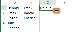
2. Now let’s copy our formula to all the cells in the column C, all the way down to the bottom row, which contains the data in the column A. To do this, move the mouse pointer to the lower right corner of the cell C1, the pointer will take the form of a black crosshair, as shown in the picture below:Click and hold down the left mouse button and drag the border of the frame down, highlighting all the cells where you want to insert the formula. When all the required cells are selected, release the mouse button:

   

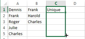
sample: In large tables, copying the formula will be faster if you use keyboard shortcuts. Highlight a cell C1 ki o si tẹ Ctrl + C (to copy the formula to the clipboard), then click Konturolu + Yipada + Ipari (to select all non-blank cells in column C) and finally press Ctrl + V (to insert the formula into all selected cells).

3. Great, now all duplicate values ​​are marked as “pidánpidán":

Option B: two columns are on different sheets (in different workbooks)

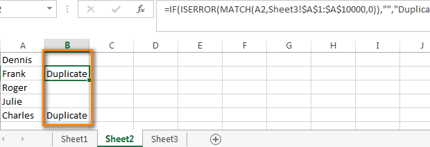
1. In the first cell of the first empty column on the worksheet Iwe 2 (in our case it is column B) enter the following formula:

   =IF(ISERROR(MATCH(A1,Sheet3!$A$1:$A$10000,0)),"","Duplicate")

   =ЕСЛИ(ЕОШИБКА(ПОИСКПОЗ(A1;Лист3!$A$1:$A$10000;0));"";"Duplicate")

   nibi Iwe 3 is the name of the sheet on which the 2nd column is located, and $A$1:$A$10000 are cell addresses from 1st to last in this 2nd column.

2. Copy the formula to all cells in a column B (same as option A).
3. A gba abajade yii:

Processing of found duplicates

Great, we have found entries in the first column that are also present in the second column. Now we need to do something with them. Going through all the duplicate records in a table manually is quite inefficient and takes too much time. There are better ways.

Show only duplicate rows in column A

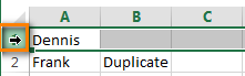
If your columns do not have headers, then you need to add them. To do this, place the cursor on the number that represents the first line, and it will turn into a black arrow, as shown in the figure below:

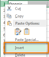
Tẹ-ọtun ko si yan lati inu akojọ aṣayan ọrọ Fi sii (Insert):

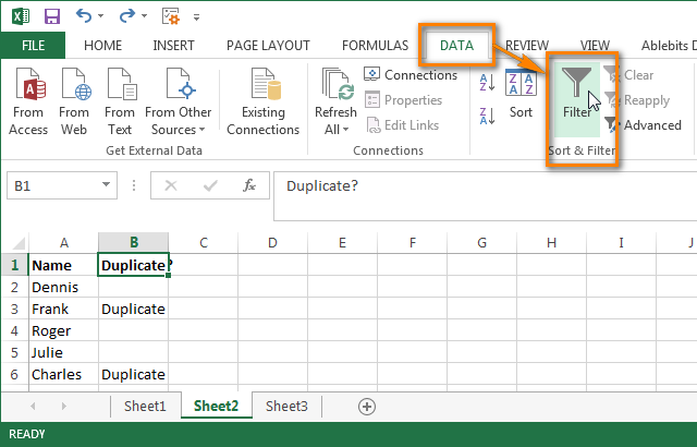
Give names to the columns, for example, “Name"Ati"Duplicate?» Then open the tab data (Data) ki o si tẹ Àlẹmọ (Filter):

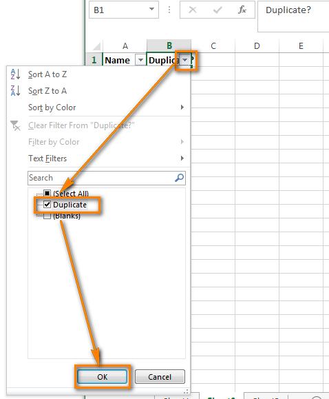
After that click on the little gray arrow next to “Duplicate?« to open the filter menu; uncheck all items in this list except pidánpidán, ki o tẹ OK.

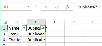
That’s all, now you see only those elements of the column А, which are duplicated in the column В. There are only two such cells in our training table, but, as you understand, in practice there will be many more of them.

To display all rows of a column again А, click the filter symbol in the column В, which now looks like a funnel with a small arrow, and select Sa gbogbo re (Select all). Or you can do the same through the Ribbon by clicking data (Data) > Select & Filter (Sort & Filter) > Clear (Clear) as shown in the screenshot below:

Change color or highlight found duplicates

If the notes “pidánpidán” is not enough for your purposes and you want to mark duplicate cells with a different font color, fill color or some other method…

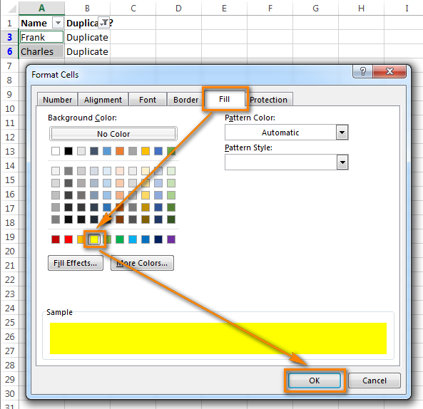
In this case, filter the duplicates as shown above, select all filtered cells and click Konturolu + 1lati ṣii ajọṣọ Awọn sẹẹli kika (cell format). As an example, let’s change the fill color of cells in rows with duplicates to bright yellow. Of course, you can change the fill color with the tool kun (Fill Color) tab Home (Home) but dialog box advantage Awọn sẹẹli kika (Cell Format) in that you can configure all the formatting options at the same time.

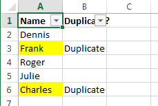
Now you will definitely not miss any cells with duplicates:

Removing duplicate values ​​from the first column

Filter the table so that only cells with duplicate values ​​are shown, and select those cells.

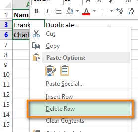
If the 2 columns you are comparing are on different sheets, that is, in different tables, right-click the selected range and select Paarẹ kana (Remove line):

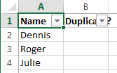
tẹ OKwhen Excel asks you to confirm that you really want to delete the entire sheet row and then clear the filter. As you can see, only rows with unique values ​​remain:

If 2 columns are on the same sheet, close to each other (adjacent) or not close to each other (not adjacent), then the process of removing duplicates will be a little more complicated. We can’t remove the entire row with duplicate values, as this will remove the cells from the second column too. So to leave only unique entries in a column А, ṣe eyi:

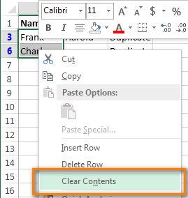
1. Filter the table to show only duplicate values ​​and select those cells. Right-click on them and select from the context menu Clear contents (clear contents).
2. Nu àlẹmọ.
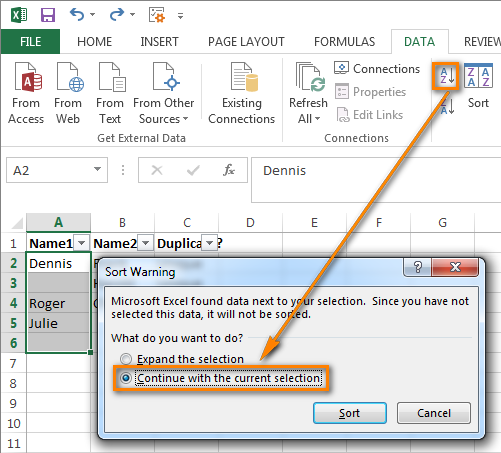
3. Yan gbogbo awọn sẹẹli ninu iwe kan А, starting from the cell A1 all the way down to the bottom containing the data.
4. tẹ awọn data (Data) ki o si tẹ To A si Z (Sort from A to Z). In the dialog box that opens, select Continue with the current selection (Sort within the specified selection) and click the button Black (Sorting):
5. Delete the column with the formula, you will no longer need it, from now on you have only unique values.
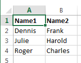
6. That’s it, now the column А contains only unique data that is not in the column В:

As you can see, removing duplicates from two columns in Excel using formulas is not that difficult.