Bii o ṣe le lorukọ sẹẹli kan ninu iwe kaakiri tayo. Bii o ṣe le lorukọ ibiti o wa ni Excel

To implement some actions in the spreadsheet, a separate identification of cells or their ranges is required. Each of them can be given a name, the assignment helps the spreadsheet processor understand where this or that element is located on the worksheet. The article will cover all the ways to give a name to a cell in a table.

N pe

You can give a name to a sector or range in a spreadsheet using several methods, which we will discuss below.

Ọna 1: okun orukọ

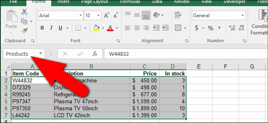
Entering the name in the name line is the easiest and most convenient method. The line of names is located to the left of the field for entering formulas. The step-by-step instruction looks like this:

1. We select a range or one sector of the table.

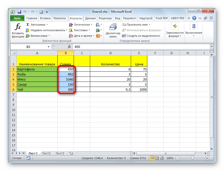
2. In the line of names we drive in the necessary name for the selected area. When entering, you must take into account the rules for assigning a name. After carrying out all the manipulations, press the “Enter” button on the keyboard.

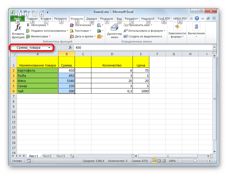
3. Ready! We have done naming a cell or a range of cells. If you select them, then the name we entered will appear in the line of names. The name of the selected area is always displayed in the name line, regardless of how the name is assigned.

Ọna 2: Akojọ ọrọ-ọrọ

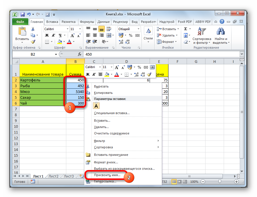
The context menu is an auxiliary component for implementing cell naming. The walkthrough looks like this:

1. We make a selection of the area to which we plan to give a name. We click RMB. A small context menu appears on the screen. We find the element “Assign a name …” and click on it.

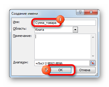
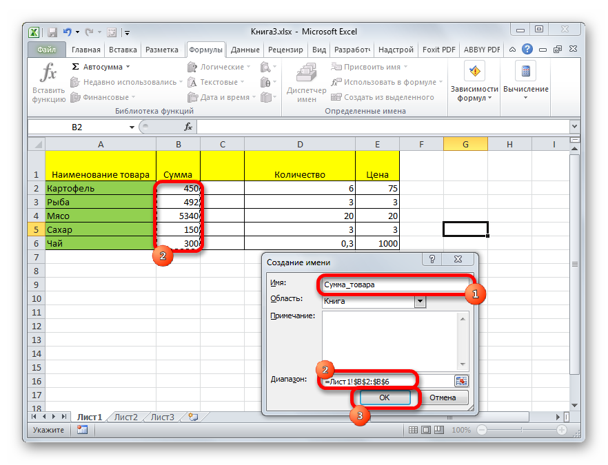
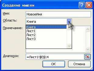
2. A new small window appeared on the screen called “Creating a Name”. In the line “Name” you must enter the name that you want to set the selected area.
3. In the line “Region” we indicate the area in which, when addressing to a given name, the selected range of sectors will be determined. The area can be either the entire document or other worksheets in the document. Usually this parameter is left unchanged.
4. The “Note” line contains completely different notes describing the selected data area. The field can be left blank as this property is not considered required.
5. In the “Range” line, enter the coordinates of the data area to which we assign a name. The coordinates of the range selected initially are placed in this line automatically.
6. Lẹhin ṣiṣe gbogbo awọn ifọwọyi, tẹ “O DARA”.

7. Ready! We gave a name to the data array using the Excel spreadsheet context menu.

Method 3: Assign a title using a button on the ribbon

With the help of special tools located on the ribbon, you can specify the name of the data area. The walkthrough looks like this:

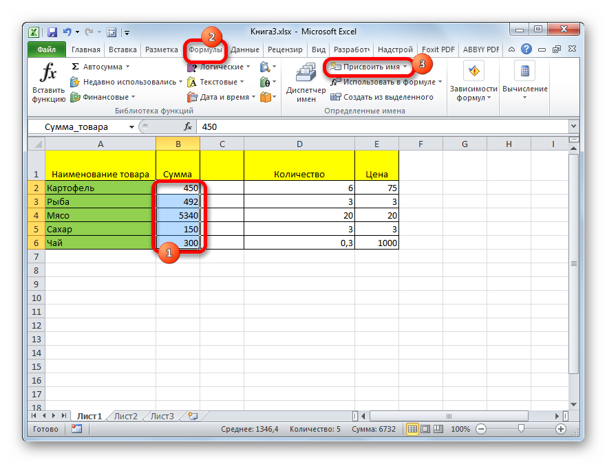
1. We make a selection of the area to which we plan to give a name. We move to the “Formulas” section. We find the block of commands “Defined names” and click on the element “Assign a name” on this panel.

2. The screen displayed a small window called “Create a name”, which we know from the previous method. We perform all the same manipulations as in the example considered earlier. Click “OK”.
3. Ready! We have assigned the name of the data area using the elements located on the tool ribbon.

Method 4: Name Manager

Through an element called “Name Manager”, you can also set a name for the selected data area. The walkthrough looks like this:

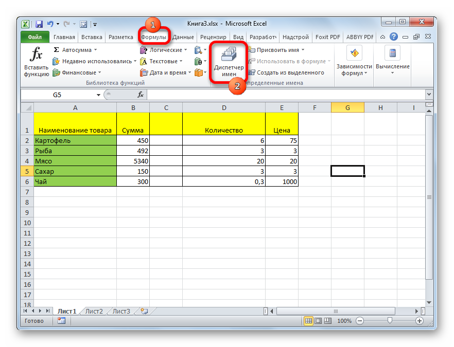
1. We move to the “Formulas” section. Find the “Defined Names” command block and click on the “Name Manager” element on this panel.

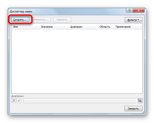
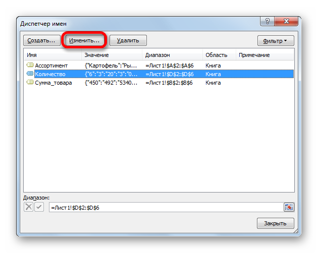
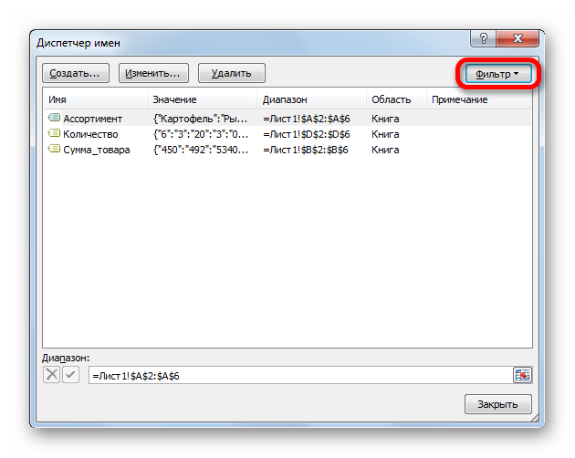
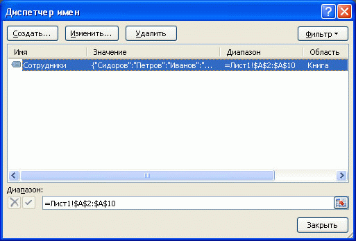
2. A small “Name Manager…” window was displayed on the display. In order to add a new name for the data area, click on the “Create …” element.

3. The display showed a familiar window called “Assign a name.” As in the methods described above, we fill in all the empty fields with the necessary information. In the line “Range” enter the coordinates of the area to assign a name. To do this, you must first click on the empty field near the inscription “Range”, and then select the desired area on the sheet itself. After carrying out all the manipulations, click on the element “OK”.

4. Ready! We assigned a name to the data area using the “Name Manager”.

Fara bale! The functionality of the “Name Manager” does not end there. The manager carries out not only the creation of names, but also allows you to manage them, as well as delete them.

The “Change…” button allows you to edit the name. To do this, you must first select an entry from the list, click on it, and then click “Edit …”. After carrying out all the actions, the user will be taken to the familiar “Assign a name” window, in which it will be possible to edit the existing parameters.

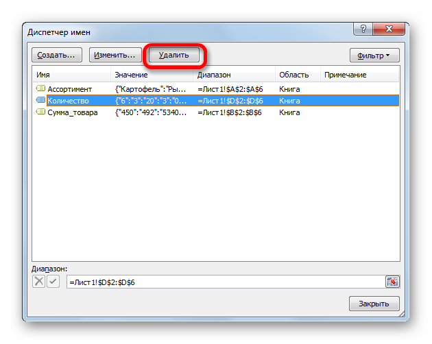
The “Delete” button allows you to delete the entry. To do this, select the desired entry, and then click on the “Delete” element.

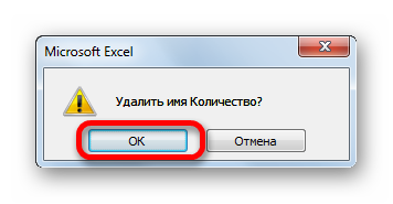
After completing these steps, a small confirmation window will appear. We click “OK”.

To all other, there is a special filter in the Name Manager. It helps users to sort and select entries from the list of titles. The use of a filter is necessary when working with a large number of titles.

Naming a Constant

Assigning a name to a constant is necessary if it has a complex spelling or frequent use. The walkthrough looks like this:

1. We move to the “Formulas” section. We find the block of commands “Defined names” and select the element “Assign a name” on this panel.
2. In the line “Name” we enter the constant itself, for example, LnPie;
3. In the line “Range” enter the following formula: =3*LN(2*ROOT(PI()))*PI()^EXP(1)

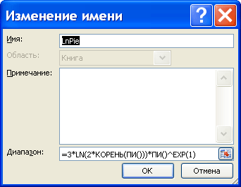
4. Ready! We have given a name to the constant.

Naming a cell and formula

You can also name the formula. The walkthrough looks like this:

1. We move to the “Formulas” section. We find the block of commands “Defined names” and click on the element “Assign a name” on this panel.
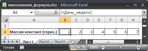
2. In the line “Name” we enter, for example, “Day_of the week”.
3. In the line “Region” we leave all the settings unchanged.
4. In the line “Range” enter ={1;2;3;4;5;6;7}.
5. Click on the “OK” element.
6. Ready! Now, if we select seven cells horizontally, we type =Day of the week in the line for formulas and press “CTRL + SHIFT + ENTER”, then the selected area will be filled with numbers from one to seven.

Naming a Range

Assigning a name to a range of cells is not difficult. The walkthrough looks like this:

1. We select the desired range of sectors.
2. We move to the “Formulas” section. We find the block of commands “Defined names” and click on the element “Create from selection” on this panel.
3. We check that the checkmark is opposite “In the line above.”
4. We click on “OK”.
5. With the help of the already familiar “Name Manager”, you can check the correctness of the name.

Naming Tables

You can also assign names to tabular data. These are tables developed with the help of manipulations carried out in the following way: Insert/Tables/Table. The spreadsheet processor automatically gives them standard names (Table1, Table2, and so on). You can edit the title using the Table Builder. The table name cannot be deleted in any way even through the “Name Manager”. The name exists until the table itself is dropped. Let’s look at a small example of the process of using a table name:

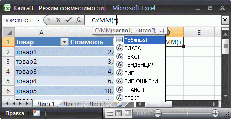
1. For example, we have a plate with two columns: Product and Cost. Outside the table, start entering the formula: =SUM(Table1[cost]).
2. At some point in the input, the spreadsheet will prompt you to select a table name.

3. After we enter =SUM(Table1[, The program will prompt you to select a field. Click “Cost”.

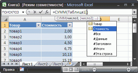
4. In the end result, we got the amount in the “Cost” column.

Syntax rules for names

The name must comply with the following syntactic rules:

• The beginning can only be a letter, a slash, or an underscore. Numbers and other special characters are not allowed.
• Spaces cannot be used in the name. They can be replaced with an underscore type.
• The name cannot be described as a cell address. In other words, it is unacceptable to use “B3: C4” in the name.
• The maximum title length is 255 characters.
• The name must be unique in the file. It is important to understand that the same letters written in uppercase and lowercase are defined as identical by the spreadsheet processor. For example, “hello” and “hello” are the same name.

Finding and checking names defined in a book

There are several methods to find and check titles in a particular document. The first method involves using the “Name Manager” located in the “Defined Names” section of the “Formulas” section. Here you can view values, comments, and sort. The second method involves the implementation of the following algorithm of actions:

1. We move to the “Formulas” section.
2. Go to the “Defined Names” block
3. Click on “Use formulas”.
4. Click “Insert Names”.
5. A window titled “Insert Name” appears on the screen. Click “All Names”. The screen will display all available titles in the document along with the ranges.

The third way involves using the “F5” key. Pressing this key activates the Jump tool, which allows you to navigate to named cells or ranges of cells.

Name Scope

Each name has its own scope. The area can be either a worksheet or the entire document as a whole. This parameter is set in the window called “Create a name”, which is located in the “Defined names” block of the “Formulas” section.

ipari

Excel offers users a huge number of options for naming a cell or a range of cells, so that everyone can choose the most convenient way to assign a name when working in a spreadsheet.