Rirọpo ọrọ olopobobo pẹlu awọn agbekalẹ

Suppose you have a list in which, with varying degrees of “straightforwardness,” initial data is written – for example, addresses or company names:

It is clearly seen that the same city or company is present here in motley variants, which, obviously, will create a lot of problems when working with these tables in the future. And if you think a little, you can find a lot of examples of similar tasks from other areas.

Now imagine that such crooked data comes to you regularly, i.e. this is not a one-time “manually fix it, forget it” story, but a problem on a regular basis and in a large number of cells.

What to do? Do not manually replace the crooked text 100500 times with the correct one through the “Find and Replace” box or by clicking Konturolu+H?

The first thing that comes to mind in such a situation is to make a mass replacement according to a pre-compiled reference book of matching incorrect and correct options – like this:

Unfortunately, with the obvious prevalence of such a task, Microsoft Excel does not have simple built-in methods for solving it. To begin with, let’s figure out how to do this with formulas, without involving “heavy artillery” in the form of macros in VBA or Power Query.

Case 1. Bulk full replacement

Let’s start with a relatively simple case – a situation where you need to replace the old crooked text with a new one. ni kikun.

Let’s say we have two tables:

In the first – the original variegated names of companies. In the second – a reference book of correspondence. If we find in the name of the company in the first table any word from the column Lati wa, then you need to completely replace this crooked name with the correct one – from the column Aropo second lookup table.

Fun irọrun:

• Both tables are converted to dynamic (“smart”) using a keyboard shortcut Konturolu+T tabi egbe Insert – Table (Insert — Table).
  
• On the tab that appears Alakoso (Apẹrẹ) first table named data, and the second reference table – Awọn ohun abuku.

To explain the logic of the formula, let’s go a little from afar.

Taking the first company from cell A2 as an example and temporarily forgetting about the rest of the companies, let’s try to determine which option from the column Lati wa meets there. To do this, select any empty cell in the free part of the sheet and enter the function there TO WA (WA):

This function determines if the given substring is included (the first argument is all values ​​from the column Lati wa) into the source text (the first company from the data table) and should output either the ordinal number of the character from which the text was found, or an error if the substring was not found.

The trick here is that since we specified not one, but several values ​​as the first argument, this function will also return as a result not one value, but an array of 3 elements. If you do not have the latest version of Office 365 that supports dynamic arrays, then after entering this formula and clicking on Tẹ you will see this array right on the sheet:

If you have previous versions of Excel, then after clicking on Tẹ we will only see the first value from the result array, i.e. error #VALUE! (#VALUE!).

You shouldn’t be afraid 🙂 In fact, our formula works and you can still see the entire array of results if you select the entered function in the formula bar and press the key F9(just don’t forget to press Escto go back to the formula):

The resulting array of results means that in the original crooked company name (GK Morozko OAO) of all values ​​in a column Lati wa found only the second (Morozko), and starting from the 4th character in a row.

Now let’s add a function to our formula Wo(WA):

Iṣẹ yii ni awọn ariyanjiyan mẹta:

1. Iye ti o fẹ – you can use any sufficiently large number (the main thing is that it exceeds the length of any text in the source data)
   
2. Viewed_vector – the range or array where we are looking for the desired value. Here is the previously introduced function TO WA, which returns an array {#VALUE!:4:#VALUE!}
   
3. Vector_awọn esi – the range from which we want to return the value if the desired value is found in the corresponding cell. Here are the correct names from the column Aropo our reference table.
   

The main and non-obvious feature here is that the function Wo if there is no exact match, always looks for the nearest smallest (previous) value. Therefore, by specifying any hefty number (for example, 9999) as the desired value, we will force Wo find the cell with the nearest smallest number (4) in the array {#VALUE!:4:#VALUE!} and return the corresponding value from the result vector, i.e. correct company name from the column Aropo.

The second nuance is that, technically, our formula is an array formula, because function TO WA returns as results not one, but an array of three values. But since the function Wo supports arrays out of the box, then we do not have to enter this formula as a classic array formula – using a keyboard shortcut Konturolu+naficula+Tẹ. A simple one will suffice Tẹ.

That’s all. Hope you get the logic.

It remains to transfer the finished formula to the first cell B2 of the column ti o wa titi – and our task is solved!

Of course, with ordinary (not smart) tables, this formula also works great (just don’t forget about the key F4 and fixing the relevant links):

Case 2. Bulk partial replacement

This case is a little trickier. Again we have two “smart” tables:

The first table with crookedly written addresses that needs to be corrected (I called it Data 2). The second table is a reference book, according to which you need to make a partial replacement of a substring inside the address (I called this table Substitutions2).

The fundamental difference here is that you need to replace only a fragment of the original data – for example, the first address has an incorrect “St. Petersburg" ni apa ọtun “St. Petersburg", leaving the rest of the address (zip code, street, house) as is.

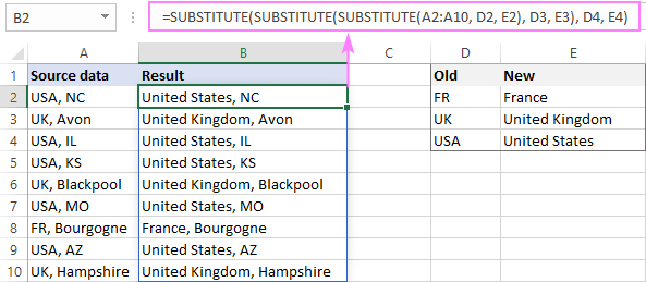
The finished formula will look like this (for ease of perception, I divided it into how many lines using alt+Tẹ):

The main work here is done by the standard Excel text function AKỌRỌ (APAPO), which has 3 arguments:

1. Source text – the first crooked address from the Address column
2. What we are looking for – here we use the trick with the function Wo (WA)from the previous way to pull the value from the column Lati wa, which is included as a fragment in a curved address.
3. What to replace with – in the same way we find the correct value corresponding to it from the column Aropo.

Enter this formula with Konturolu+naficula+Tẹ is not needed here either, although it is, in fact, an array formula.

And it is clearly seen (see #N/A errors in the previous picture) that such a formula, for all its elegance, has a couple of drawbacks:

• iṣẹ SUBSTITUTE is case sensitive, so “Spb” in the penultimate line was not found in the replacement table. To solve this problem, you can either use the function ZAMENIT (PARAPA), or preliminarily bring both tables to the same register.
• If the text is initially correct or in it there is no fragment to replace (last line), then our formula throws an error. This moment can be neutralized by intercepting and replacing errors using the function IFEROR (IFERROR):

  

• If the original text contains several fragments from the directory at once, then our formula replaces only the last one (in the 8th line, Ligovsky «Avenue« yipada si “pr-t”, Sugbon “S-Pb” on “St. Petersburg" no longer, because “S-Pb” is higher in the directory). This problem can be solved by re-running our own formula, but already along the column ti o wa titi:

  
  

Not perfect and cumbersome in places, but much better than the same manual replacement, right? 🙂

PS

In the next article, we will figure out how to implement such a bulk substitution using macros and Power Query.

• How the SUBSTITUTE function works to replace text
  
• Finding Exact Text Matches Using the EXACT Function
• Case sensitive search and substitution (case sensitive VLOOKUP)