Isọdi awọn shatti ni Excel: fifi akọle kun, awọn aake, arosọ

What is the first thing you do after creating a chart in Excel? Naturally, arrange it so that it matches the picture that your imagination has drawn.

In recent versions of spreadsheets, customizing charts is a pretty nice and easy process.

Microsoft has gone to great lengths to simplify the customization process. For example, she put the necessary buttons in places where it is most convenient to reach them. And later in this tutorial, you will learn a series of simple methods for adding and modifying all the elements of charts and graphs in Excel.

Three Easy Customization Methods

If you know how to create graphs in Excel, you know that you can access its settings in three ways:

1. Select chart and jump to section "Nṣiṣẹ pẹlu awọn apẹrẹ", eyi ti o le ri lori taabu "Olukole".
2. Right-click on the element that needs to be changed and select the desired item from the pop-up menu.
3. Use the chart customization button displayed in the upper right corner of the chart after clicking on it with the left button.

If you need to configure more options that allow you to edit the appearance of the graph, you can see them in the area indicated by the heading “Fọọmu agbegbe Chart”, which can be accessed by clicking on the item "Awọn aṣayan afikun" in the popup menu. You can also see this option in the group "Nṣiṣẹ pẹlu awọn apẹrẹ".

To immediately display the “Format Chart Area” panel, you can double-click on the required element.

Now that we’ve covered the basic required information, let’s figure out how to change the different elements to make the chart look the way we want it to.

How to add a title

Since most people use the latest versions of spreadsheets, it would be a good idea to look at how to add a header in Excel 2013 and 2016. 

How to add a title to a chart in Excel 2013 and 2016

In these versions of spreadsheets, the title is already automatically inserted into the chart. To edit it, just click on it and write the required text in the input field.

You can also locate the heading in a specific cell in the document. And, if the linked cell is updated, the name changes after it. You will learn more about how to achieve this result later.

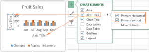
If the title was not created by the program, then you must click on any place in the chart to display the tab "Nṣiṣẹ pẹlu awọn apẹrẹ". Next, select the “Design” tab and click on “Add Chart Element”. Next, you need to select the title and indicate its location as shown in the screenshot.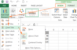

You can also see a plus sign in the upper right corner of the chart. If you click on it, a list of elements available in the diagram appears. To display the title, you must check the box next to the corresponding item.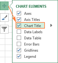

Alternatively, you can click on the arrow next to "Akọle chart" ki o si yan ọkan ninu awọn aṣayan wọnyi:

1. Above the diagram. This is the default value. This item displays the title at the top of the chart and resizes it.
2. Center. In this case, the chart does not change its size, but the title is superimposed on the chart itself.

To configure more parameters, you need to go to the tab "Olukole" and follow these options:

1. Add a chart element.
2. Title of the chart.
3. Additional header options.

You can also click on the icon "Awọn eroja apẹrẹ", ati igba yen - "Akọle chart" и "Awọn aṣayan afikun". In any case, a window opens “Chart Title Format”ti salaye loke.

Header customization in Excel 2007 and 2010 versions

To add a title in Excel 2010 and below, follow these steps:

1. Tẹ nibikibi lori chart.
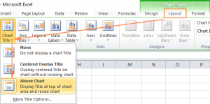
2. A group of tabs will appear at the top. "Nṣiṣẹ pẹlu awọn apẹrẹ", where you need to select an item “Ìfilélẹ̀”. There you should click on "Akọle chart".
3. Next, you need to select the desired location: in the upper part of the plotting area or overlaying the title on the chart.

Linking a header to a specific cell in a document

For the vast majority of chart types in Excel, the newly created chart is inserted along with a title pre-written by programmers. It should be replaced with your own. You need to click on it and write the necessary text. It is also possible to link it to a specific cell in the document (the name of the table itself, for example). In this case, the chart title will be updated when you edit the cell it is associated with.

To connect a header to a cell, follow these steps:

1. Yan akọle kan. 
2. In the formula input field, you must write =, click on the cell containing the required text, and press the “Enter” button.

In this example, we have connected the title of the chart showing fruit sales to cell A1. It is also possible to select two or more cells, for example, a pair of column headings. You can make them appear in the title of the graph or chart.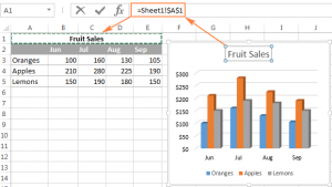

How to move the title

If you need to move the title to another part of the graph, you need to select it and move it with the mouse.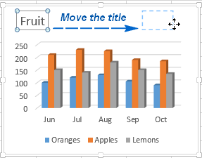

Removing a title

If you do not need to add a title to the chart, then you can remove the title in two ways:

1. Lori To ti ni ilọsiwaju taabu "Olukole" successively click on the following items: “Add Chart Elements” - "Akọle chart" - “Not”.
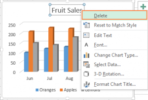
2. Right-click on the title and call the context menu in which you need to find the item "Paarẹ".

Header Formatting

To correct the font type and color of the name, you need to find the item in the context menu "Fọnti". A corresponding window will appear where you can set all the necessary settings.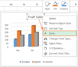

If you need more subtle formatting, you need to click on the title of the graph, go to the tab "Ọna kika" and change the settings as you see fit. Here is a screenshot demonstrating the steps to change the title font color via the ribbon.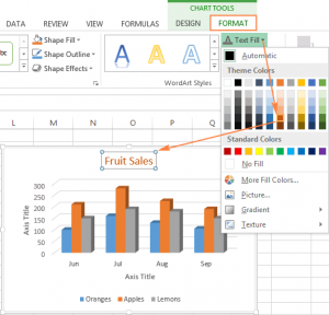

By a similar method, it is possible to modify the formation of other elements, such as the legend, axes, titles.

Chart axis customization

Usually the vertical (Y) and horizontal (X) axes are added at once when you create a graph or chart in Excel.

You can show or hide them using the “+” button in the upper right corner and click on the arrow next to “Axes”. In the window that appears, you can select those that should be displayed and those that are better hidden.

In some types of graphs and charts, an additional axis can also be displayed.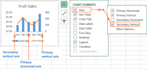

If you need to create a XNUMXD chart, you can add a depth axis.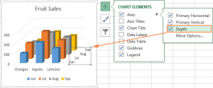

The user can define how different axes will be displayed on the Excel chart. The detailed steps are described below.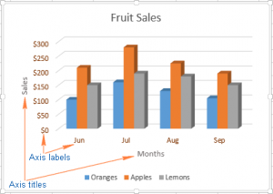

Adding Axis Titles

To help the reader understand the data, you can add labels for the axes. To do this, do the following:

1. Click on the diagram, then select the item "Awọn eroja apẹrẹ" ati ki o ṣayẹwo apoti “Axis Names”. If you want to specify a title only for a specific axis, you need to click on the arrow and clear one of the checkboxes.
2. Click on the axis title input field and enter the text.

To define the appearance of the title, right-click and find the “Axis Title Format” item. Next, a panel will be shown in which all possible formatting options are configured. It is possible to try different options for displaying the title on the tab "Ọna kika", as shown above when it came to changing the title format.

Associating an axis title with a specific document cell

Just like with chart titles, you can bind an axis title to a specific cell in the document so that it updates as soon as the corresponding cell in the table is edited.

To bind a title, you must select it, write = in the appropriate field and select the cell that you want to bind to the axis. After these manipulations, you need to click on the “Enter” button.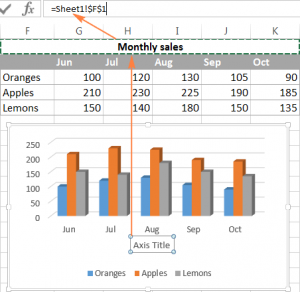

Change the scale of the axes

Excel itself finds the largest and smallest value, depending on the data entered by the user. If you need to set other parameters, you can do it manually. You need to do the following:

1. Select the x-axis of the chart and click on the icon "Awọn eroja apẹrẹ".
2. Click on the arrow icon in the row “Axis” and in the pop-up menu click on "Awọn aṣayan afikun".
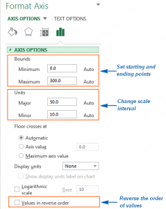
3. Next comes the section “Axis Options”where any of these actions are performed:
   1. To set the start and end values ​​of the Y axis, you must specify it in the fields “Minimum” and “Maximum”.
   2. To change the scale of the axis, you can also specify values ​​in the field “Basic divisions” и “Intermediate divisions”.
   3. To configure the display in reverse order, you need to check the box next to the option “Ipaṣẹ Yipada ti Awọn iye”.

Since the horizontal axis usually displays text labels, it has less customization options. But you can edit the number of categories displayed between the labels, their sequence and where the axes intersect.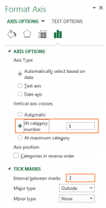

Changing the Format of Axis Values

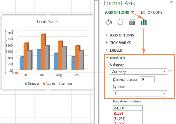
If you need to display the values ​​on the axes as a percentage, time, or any other format, you must select the item from the pop-up menu. “Format Axis”, and in the right part of the window, select one of the possible options where it says "Nọmba".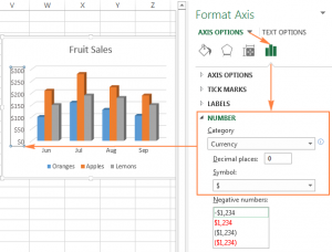

Iṣeduro: to configure the format of the initial information (that is, the values ​​indicated in the cells), you must check the box next to the item “Link to Source”. If you can’t find the section "Nọmba" in the panel “Format Axis”, you need to make sure that you have previously selected the axis that displays the values. Usually it is the X axis.

Adding Data Labels

To make the chart easier to read, you can add labels to the data you provide. You can add them to one row or to all. Excel also provides the ability to add labels only to certain points.

To do this, you need to follow these steps:

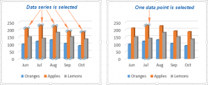
1. Click on the data series requiring signatures. If you want to mark only one point with text, you need to click on it again.
2. Tẹ aami naa "Awọn eroja apẹrẹ" ati ṣayẹwo apoti ti o tẹle "Awọn Ibuwọlu Data".

For example, here is what one of the charts looks like after labels have been added to one of the data series in our table.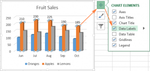

For specific types of charts (such as pie charts), you can specify the location of the label. To do this, click on the arrow next to the line "Awọn Ibuwọlu Data" and indicate a suitable location. To display labels in floating input fields, you must select the item "Ipe data". If you need more settings, you can click on the corresponding item at the very bottom of the context menu.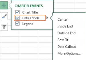

How to change the content of signatures

To change the data displayed in the signatures, you must click on the button "Awọn eroja apẹrẹ" - "Awọn Ibuwọlu Data" - "Awọn aṣayan afikun". The panel will then appear. "Iwe kika aami data". There you need to go to the tab "Awọn aṣayan Ibuwọlu" in and select the desired option in the section "Fi sinu Ibuwọlu".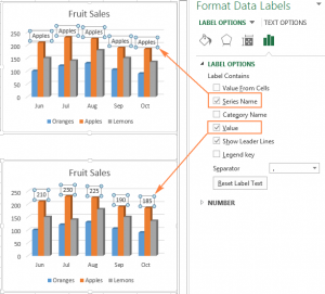

If you want to add your own text to a particular data point, you must double-click on the corresponding label so that only it is selected. Next, select a label with existing text and enter the text you want to replace.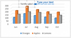

If you decide that too many labels are displayed in the chart, you can remove any of them by right-clicking on the corresponding label and clicking on the button "Paarẹ" ninu akojọ aṣayan ti o han.

Some guidelines for defining data labels:

1. To change the location of the signature, you need to click on it and move it to the desired location with the mouse.
2. To edit the background color and signature font, select them, go to the tab "Ọna kika" and set the required parameters.

Legend setup

After you create a chart in Excel, the legend will automatically appear at the bottom of the chart if Excel version is 2013 or 2016. If an earlier version of the program is installed, it will be displayed on the right side of the plot area.

To hide the legend, you must click on the button with a plus sign in the upper right corner of the chart and uncheck the corresponding box.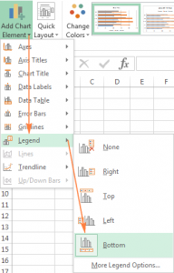

To move it, you need to click on the diagram, move to the tab "Olukole" ki o si tẹ “Add Chart Element” and select the required position. You can also delete the legend through this menu by clicking on the button “Not”. 

You can also change the location by double-clicking on it and in the options (on the right side of the screen) selecting the desired location.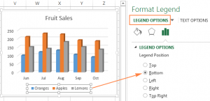

To change the formatting of the legend, there are a huge number of settings in the tab “Shading and borders”, "Awọn ipa" ni ọtun nronu.

How to show or hide the grid of an Excel document

The grid is shown or hidden using the same pop-up menu used to show the title, legend, and other chart elements.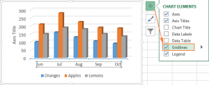

The program will automatically select the most suitable grid type for a particular chart. If you need to change it, you should click on the arrow next to the corresponding item and click on "Awọn aṣayan afikun".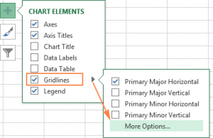

Hiding and editing data series in Excel

To hide or edit individual data series in Excel, you must click the button on the right side of the graph “Chart Filters” and remove unnecessary checkboxes. 

To edit the data, click on “Change Row” on the right side of the title. To see this button, you need to hover over the row name.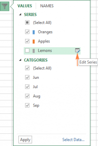

Yi awọn chart iru ati ara

To change the chart type, you need to click on it, go to the tab "Fi sii" ati ni apakan "Awọn aworan atọka" choose the appropriate type.

You can also open the context menu and click on "Yipada Iru iwe apẹrẹ".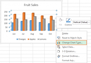

To quickly change the chart style, you must click on the corresponding button (with a brush) to the right of the chart. You can select the appropriate one from the list that appears.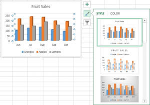

You can also select the appropriate style in the section "Awọn aṣa apẹrẹ" ninu taabu "Olukole".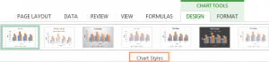

Change chart colors

To edit the color scheme, click on the button "Awọn aṣa apẹrẹ" and in tab "Awọ" choose an appropriate topic.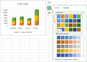

You can also use the tab "Ọna kika"where to click the button "kun apẹrẹ".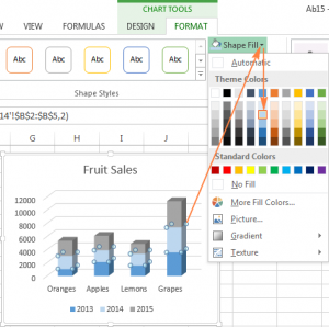

How to understand the places of the axis

To achieve this goal, it is necessary on the tab "Olukole" Titari bọtini “Row column”.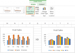

Chart spread from left to right

To rotate the chart from left to right, you need to right-click on the horizontal axis and click “Format Axis”.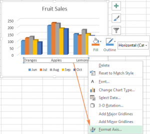

You can also in the tab "Olukole" find item “Additional Axis Options”.

In the right panel, select the item “Ipaṣẹ yipo awọn ẹka”.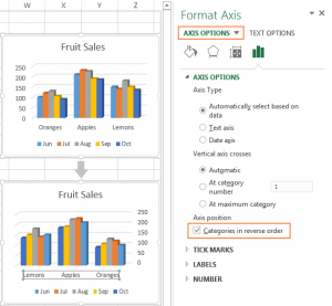

There are also a number of other possibilities, but it is impossible to consider everything. But if you learn how to use these features, it will be much easier to learn new ones yourself. Good luck!