Awọn ọwọn farasin ni Excel. Awọn ọna 3 lati ṣafihan Awọn ọwọn Farasin ni Excel

Often when using the spreadsheet editor, there are times when it is necessary that specific columns of the table be hidden. As a result of these actions, the necessary columns are hidden, and they are no longer visible in the spreadsheet document. However, there is also an inverse operation – expanding columns. In the article, we will consider in detail several methods for implementing this procedure in a spreadsheet editor.

Showing Hidden Columns in the Table Editor

Hiding columns is a handy tool that allows you to correctly position elements on the workspace of a spreadsheet document. This function is often used in the following cases:

1. The user wants to compare two columns separated by other columns. For example, you need to compare column A and column Z. In this case, it will be convenient to perform the procedure for hiding interfering columns.
2. The user wants to hide a number of additional auxiliary columns with calculations and formulas that prevent him from conveniently working with information located in the workspace of a spreadsheet document.
3. The user wants to hide some columns of a spreadsheet document so that they do not interfere with the viewing of tabular information by other users who will work in this document.

Now let’s talk about how to implement the opening of hidden columns in the Excel spreadsheet editor.

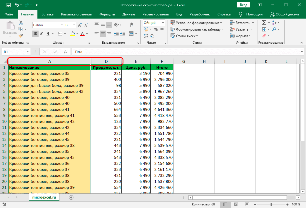
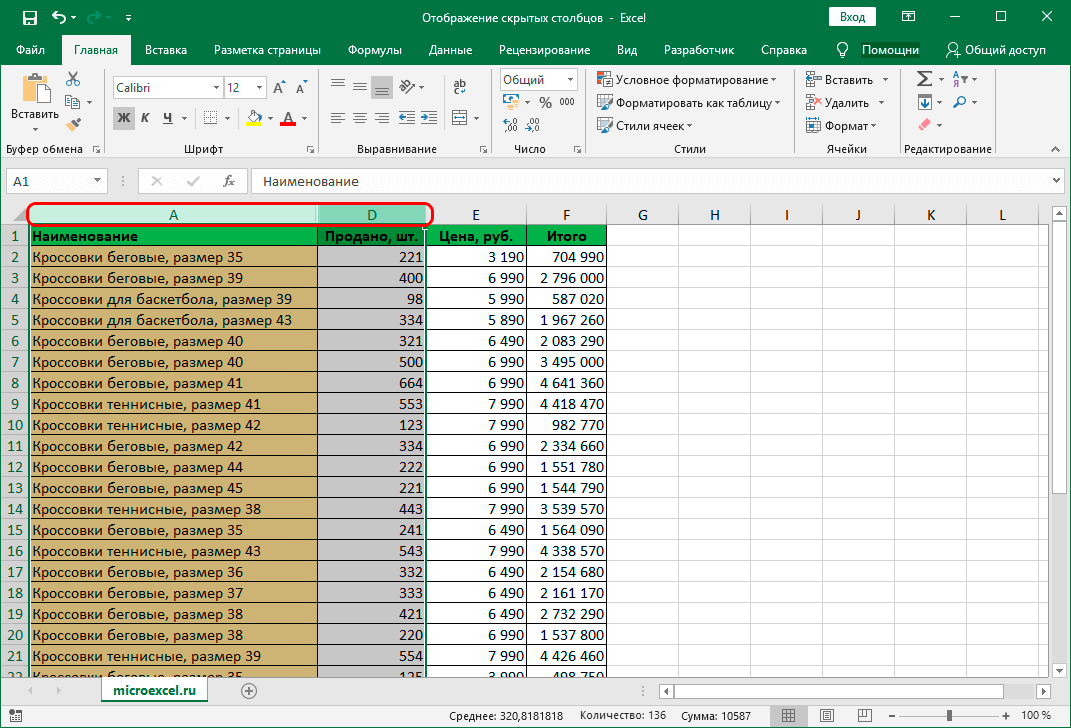
Initially, you need to make sure that there are hidden columns in the plate, and then determine their location. This procedure is easily implemented using the horizontal coordinate bar of the spreadsheet editor. It is necessary to carefully look at the sequence of names, if it is violated, then in this location there is a hidden column or several columns.

After we have found out that there are hidden components in the spreadsheet document, it is necessary to perform the procedure for their disclosure. This procedure can be implemented in several ways.

First way: moving cell borders

Detailed instructions for moving cell borders in a spreadsheet document look like this:

1. Move the pointer to the column border. The cursor will take the form of a small black line with arrows pointing in opposite directions. By holding down the left mouse button, we drag the borders in the required direction.

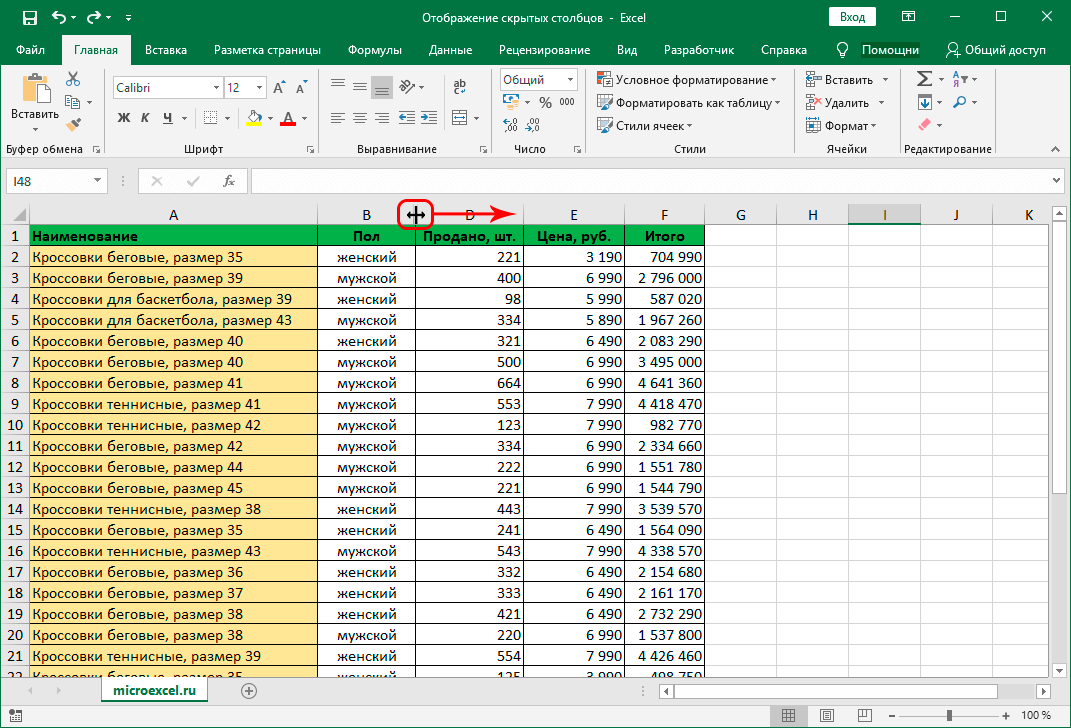
2. This simple procedure allows you to make the column labeled “C” visible. Ready!

Pataki! This method is very easy to use, but if there are too many hidden columns in a spreadsheet document, then this procedure will need to be performed a huge number of times, which is not very convenient, in which case it is more expedient to apply the methods that we will discuss later.

The second way: using a special context menu

This method is the most common among spreadsheet editor users. It, like the one above, allows you to implement the disclosure of hidden columns. Detailed instructions for using a special context menu in a spreadsheet document look like this:

1. By holding down the left mouse button, we select the range of columns on the coordinate panel. You need to select those cells in which the hidden columns are located. You can select the entire workspace using the Ctrl + A button combination.

2. Right-click anywhere in the selected range. A large list appeared on the screen, allowing you to perform various transformations in the selected area. We find the element with the name “Show”, and click on it with the left mouse button.

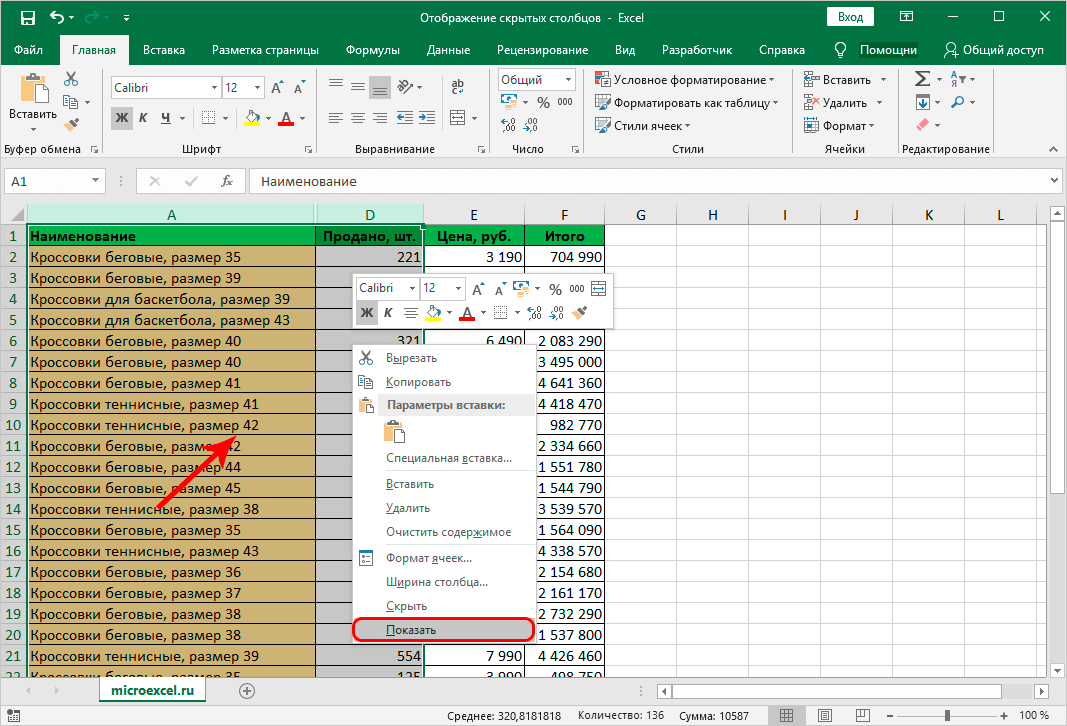
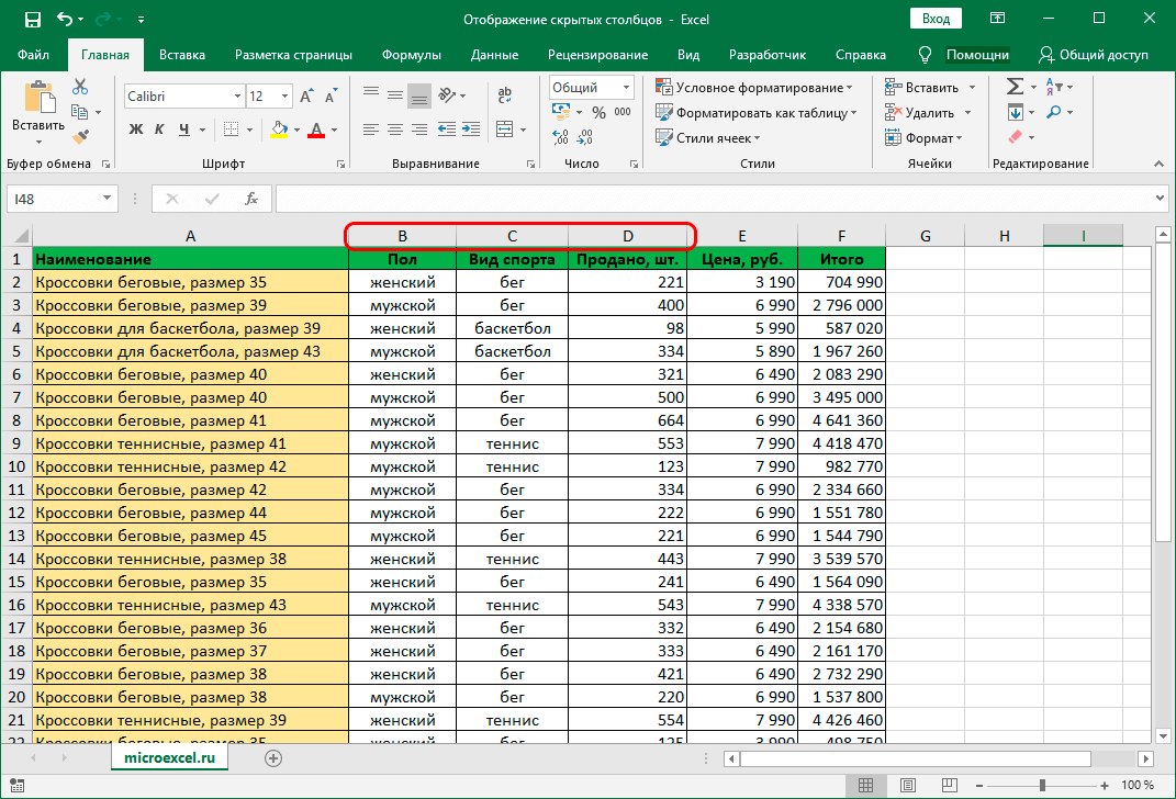
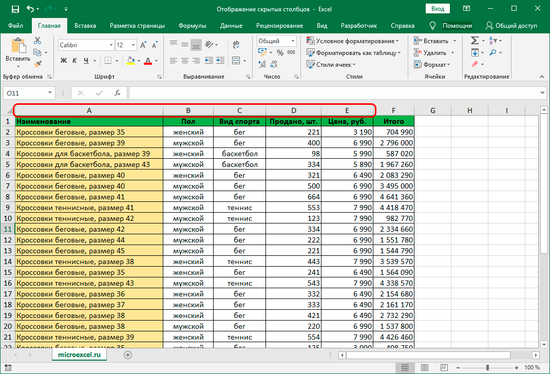
3. As a result, all hidden columns in the selected range will be displayed in a spreadsheet document. Ready!

The third way: using elements on a special ribbon

This method involves the use of a special ribbon on which the spreadsheet editor tools are located. Detailed instructions for using the tools on the special ribbon of the spreadsheet editor look like this:

1. By holding down the left mouse button, we select the range of columns on the coordinate panel. You need to select those cells in which the hidden columns are located.
2. You can select the entire workspace using the Ctrl + A combination.
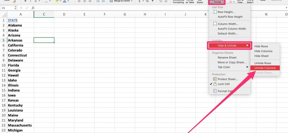
3. We move to the “Home” subsection, find the “Cells” block of elements there, and then click the left mouse button on “Format”. A small list has opened, in which you need to select the “Hide or show” item, which is located in the “Visibility” block. In the next list, select the item “Show columns” with the left mouse button.

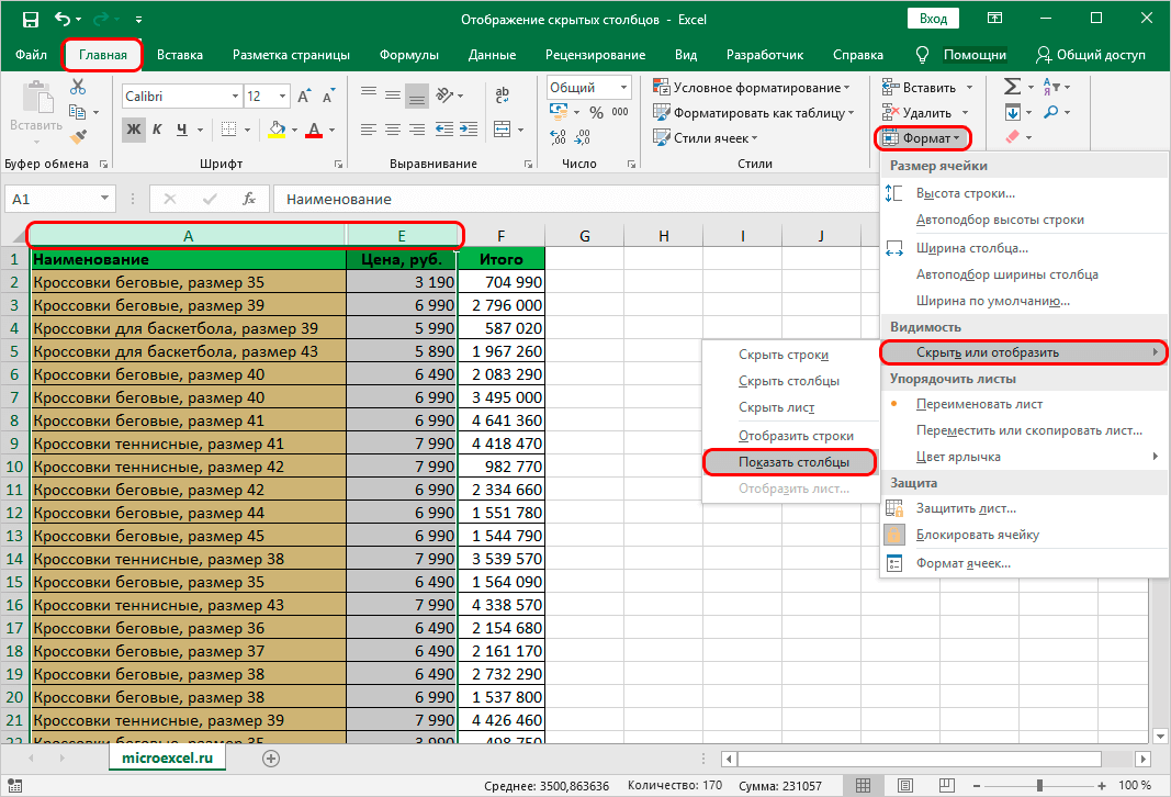
4. Ready! Hidden columns are displayed again in the spreadsheet workspace.

Conclusion and conclusions about the display of hidden columns in the spreadsheet editor

Hiding columns is a handy feature that allows you to temporarily hide specific information from the spreadsheet document workspace. This procedure allows you to make a spreadsheet document more convenient and comfortable to use, especially in cases where the document contains a huge amount of information. However, not everyone knows how to implement the procedure for revealing hidden columns in a spreadsheet document. We have examined in detail three ways to implement the display of hidden elements of the workspace of a spreadsheet document, so that each user can choose the most convenient method for himself.