Awọn ọna 2 lati Yi abẹlẹ pada ni Excel

In this article, you will learn two simple ways to change the background of cells based on their content in the latest versions of Excel. You will also understand which formulas to use to change the shade of cells or cells where the formulas are written incorrectly, or where there is no information at all.

Everyone knows that editing the background of a simple cell is a simple procedure. Click on “background color”. But what if you need color correction based on a certain cell content? How can I make this happen automatically? What follows is a series of useful information that will enable you to find the right way to accomplish all of these tasks.

Dynamic cell background color change

Išẹ: You have a table or set of values, and you need to edit the background color of the cells based on what number is entered there. You also need to ensure that the hue responds to changing values.

ojutu: For this task, Excel’s “conditional formatting” function is provided to color cells with numbers greater than X, less than Y, or between X and Y.

Let’s say you have a set of products in different states with their prices, and you need to know which of them cost more than $3,7. Therefore, we decided to highlight those products that are above this value in red. And cells that have a similar or greater value, it was decided to stain in a green tint.

akiyesi: The screenshot was taken in the 2010 version of the program. But this does not affect anything, since the sequence of actions is the same, regardless of which version – the latest or not – the person uses.

So here’s what you need to do (step by step):

1. Select the cells in which the hue should be edited. For example, the range $B$2:$H$10 (column names and the first column, which lists state names, are excluded from the sample).

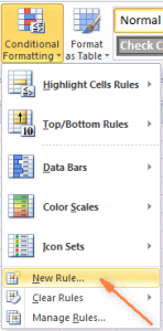
2. Tẹ lori "Ile" ninu ẹgbẹ "ara". There will be an item “Conditional Formatting”. There you also need to select “New Rule”. In the English version of Excel, the sequence of steps is as follows: “Home”, “Styles group”, “Conditional Formatting > New Rule».

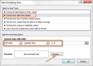
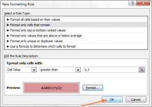
3. In the window that opens, check the box “Format only cells that contain” (“Format only cells that contain” in the English version).

4. At the bottom of this window under the inscription “Format only cells that meet the following condition” (Format only cells with) you can assign rules by which formatting will be performed. We have chosen the format for the specified value in cells, which must be greater than 3.7, as you can see from the screenshot: 

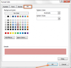
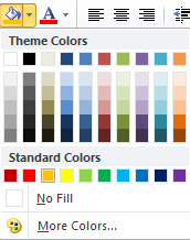
5. Next, click on the button "Ọna kika". A window will appear with a background color selection area on the left. But before that, you need to open the tab "Fi kun" («Fill»). In this case, it’s red. After that, click on the “OK” button.

6. Then you will return to the window “New Formatting Rule”, but already at the bottom of this window you can preview how this cell will look like. If everything is fine, you need to click on the “OK” button.

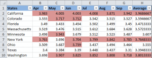
As a result, you get something like this:

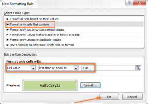
Next, we need to add one more condition, that is, change the background of cells with values ​​less than 3.45 to green. To perform this task, you must click on “New Formatting Rule” and repeat the steps above, only the condition needs to be set as “less than, or equivalent” (in the English version “less than or equal to”, and then write the value. At the end, you need to click the “OK” button.

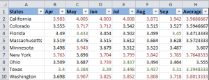
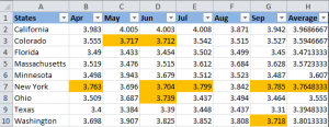
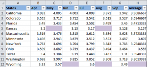
Now the table is formatted in this way.

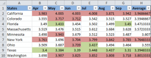
It displays the highest and lowest fuel prices in various states, and you can immediately determine where the situation is most optimistic (in Texas, of course).

Iṣeduro: If necessary, you can use a similar formatting method, editing not the background, but the font. To do this, in the formatting window that appeared in the fifth stage, you need to select the tab "Fọnti" and follow the prompts given in the window. Everything is intuitively clear, and even a beginner can figure it out.

As a result, you will get a table like this:

How to keep cell color the same even if value changes?

Išẹ: You need to color the background so that it never changes, even if the background changes in the future.

ojutu: find all cells with specific number using excel function “Find all” “Find All” or add-on “Select special cells” (“Select Special Cells”), and then edit the cell format using the function “Format cells” («Format Cells»).

This is one of those infrequent situations that are not covered in the Excel manual, and even on the Internet, the solution to this problem can be found quite rarely. Which is not surprising, since this task is not standard. If you want to edit the background permanently so that it never changes until it is manually adjusted by the user of the program, you must follow the instructions above.

Select all cells that contain a certain condition

There are several possible methods, depending on what kind of particular value is to be found.

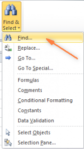
If you need to designate cells with a specific value with a special background, you need to go to the tab "Ile" ati yan “Find and select” – “Find”.

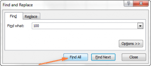
Enter the required values ​​and click on “Find All”.

Egba Mi O: You can click on the button “Awọn aṣayan” on the right to take advantage of some additional settings: where to search, how to view, whether to respect uppercase and lowercase letters, and so on. You can also write additional characters, such as an asterisk (*), to find all lines containing these values. If you use a question mark, you can find any single character.

In our previous example, if we wanted to find all fuel quotes between $3,7 and $3,799, we could refine our search query.

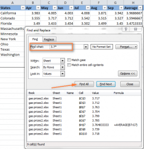
Now select any of the values ​​that the program found at the bottom of the dialog box and click on one of them. After that, press the key combination “Ctrl-A” to select all the results. Next, click on the “Close” button. 

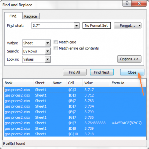
Here’s how to select all cells with specific values ​​using the Find All feature. In our example, we need to find all fuel prices above $3,7, and unfortunately Excel does not allow you to do this using the Find and Replace function.

The “barrel of honey” comes to light here because there is another tool that will help with such complex tasks. It’s called Select Special Cells. This add-on (which needs to be installed to Excel separately) will help:

• find all values ​​in a certain range, for example between -1 and 45,
• get the maximum or minimum value in a column,
• find a string or range,
• find cells by background color and much more.

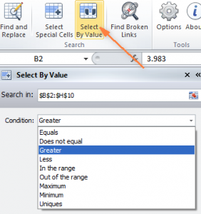
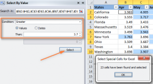
After installing the add-on, simply click the button “Select by value” (“Select by Value”) and then refine the search query in the addon window. In our example, we are looking for numbers greater than 3,7. Press "Yan" (“Select”), and in a second you will get a result like this:

If you are interested in the add-on, you can download a trial version at asopọ.

Changing the background of selected cells through the “Format Cells” window

Now, after all the cells with a certain value have been selected using one of the methods described above, it remains to specify the background color for them.

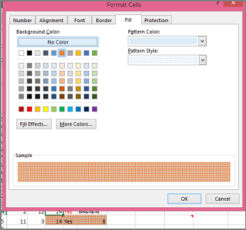
To do this, you need to open a window “Cell format”by pressing the Ctrl + 1 key (you can also right-click on the selected cells and left-click on the “cell formatting” item) and adjust the formatting that you need.

We will choose an orange shade, but you can choose any other.

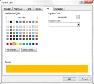
If you need to edit the background color without changing other appearance parameters, you can simply click on “color fill” and choose the color that suits you perfectly.

The result is a table like this:

Unlike the previous technique, here the color of the cell will not change even if the value is edited. This can be used, for example, to track the dynamics of goods in a certain price group. Their value has changed, but the color has remained the same.

Editing the background color for special cells (blank or with errors when writing a formula)

Similar to the previous example, the user has the ability to edit the background color of special cells in two ways. There are static and dynamic options.

Applying a Formula to Edit a Background

Here the color of the cell will be edited automatically based on its value. This method helps users a lot and is in demand in 99% of situations.

As an example, you can use the previous table, but now some of the cells will be empty. We need to determine which ones do not contain any readings and edit the background color.

1. On the tab "Ile" you need to click on “Conditional Formatting” ->  “New Rule” (same as in step 2 of the first section “Change the background color dynamically”.

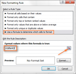
2. Next, you need to select the item “Use a formula to determine…”.

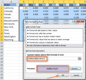
3. Enter formula =IsBlank() (ISBLANK in the version), if you want to edit the background of an empty cell, or =IsError() (ISERROR in the version), if you need to find a cell where there is an erroneously written formula. Since in this case we need to edit empty cells, we enter the formula =IsBlank(), and then place the cursor between the parentheses and click on the button next to the formula input field. After these manipulations, a range of cells should be manually selected. In addition, you can specify the range yourself, for example, =IsBlank(B2:H12).

4. Click on the “Format” button and select the appropriate background color and do everything as described in paragraph 5 of the “Dynamic cell background color change” section, and then click “OK”. There you can also see what the color of the cell will be. The window will look something like this.

5. If you like the background of the cell, you must click on the “OK” button, and the changes will be immediately made to the table.

Static change of background color of special cells

In this situation, once assigned, the background color will continue to remain that way, no matter how the cell changes.

If you need to permanently change special cells (empty or containing errors), follow these instructions:

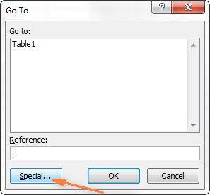
1. Select your document or several cells and press F5 to open the Go To window, and then press the button “Highlight”.
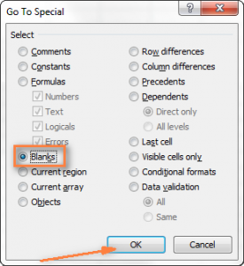
2. In the dialog box that opens, select the “Blanks” or “Empty cells” button (depending on the version of the program – or English) to select empty cells.
3. If you need to highlight cells that have formulas with errors, you should select the item "Awọn agbekalẹ" and leave a single checkbox next to the word “Errors”. As follows from the screenshot above, cells can be selected according to any parameters, and each of the described settings is available if necessary.
4. Finally, you need to change the background color of the selected cells or customize them in any other way. To do this, use the method described above.

Just remember that formatting changes made this way will persist even if you fill in gaps or change the special cell type. Of course, it is unlikely that someone will want to use this method, but in practice anything can happen.

How to get the most out of Excel?

As heavy users of Microsoft Excel, you should know that it contains many features. Some of them we know and love, while others remain mysterious to the average user, and a large number of bloggers are trying to shed at least a little light on them. But there are common tasks that each of us will have to perform, and Excel does not introduce some features or tools to automate some complex actions.

And the solution to this problem is add-ons (addons). Some of them are distributed free of charge, others – for money. There are many similar tools that can perform different functions. For example, find duplicates in two files without cryptic formulas or macros.

If you combine these tools with the core functionality of Excel, you can achieve very great results. For example, you can find out which fuel prices have changed, and then find duplicates in the file for the past year.

We see that conditional formatting is a handy tool that allows you to automate work on tables without any specific skills. You now know how to fill cells in several ways, based on their contents. Now it remains only to put it into practice. Good luck!