Bii o ṣe le ṣe atokọ sisọ silẹ ni Excel

The drop-down list is an incredibly useful tool that can help make working with information more comfortable. It makes it possible to contain several values ​​​​in a cell at once, with which you can work, like with any others. To select the one you need, just click on the arrow icon, after which a list of values ​​uXNUMXbuXNUMXbis displayed. After selecting a specific one, the cell is automatically filled with it, and the formulas are recalculated based on it.

Excel provides many different methods for generating a drop-down menu, and in addition, it allows you to flexibly customize them. Let’s analyze these methods in more detail.

List creation process

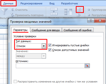
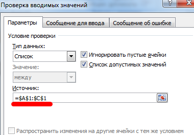
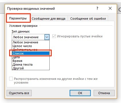
To generate a pop-up menu, click on the menu items along the path “Data” – “Data Validation”. A dialog box will open where you need to find the “Parameters” tab and click on it if it has not been opened before. It has a lot of settings, but the “Data Type” item is important to us. Of all the meanings, “List” is the right one.

The number of methods by which information is entered into the pop-up list is quite large.

1. Independent indication of list elements separated by a semicolon in the “Source” field located on the same tab of the same dialog box.
   

   

2. Preliminary indication of values. The Source field contains the range where the required information is available.
   

   

3. Specifying a named range. A method that repeats the previous one, but it is only necessary to preliminarily name the range.
   

   

Any of these methods will produce the desired result. Let’s look at methods for generating drop-down lists in real-life situations.

Based on data from the list

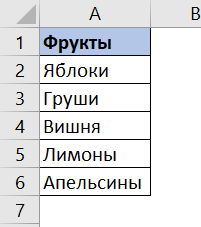
Let’s say we have a table describing the types of different fruits.

To create a list in a drop-down menu based on this set of information, you need to do the following:

1. Select the cell reserved for the future list.
2. Find the Data tab on the ribbon. There we click on “Verify data”.
   

   

3. Find the item “Data Type” and switch the value to “List”.
   

   

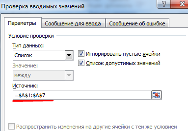
4. In the field denoting the “Source” option, enter the desired range. Please note that absolute references must be specified so that when copying the list, the information does not shift.
   

In addition, there is a function to generate lists at once in more than one cell. To achieve this, you should select them all, and perform the same steps as described earlier. Again, you need to make sure that absolute references are written. If the address does not have a dollar sign next to the column and row names, then you need to add them by pressing the F4 key until the $ sign is next to the column and row names.

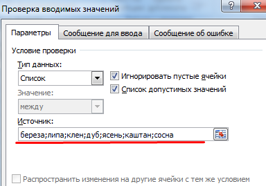
With manual data recording

In the situation above, the list was written by highlighting the required range. This is a convenient method, but sometimes it is necessary to manually record the data. This will make it possible to avoid duplication of information in the workbook.

Suppose we are faced with the task of creating a list containing two possible choices: yes and no. To accomplish the task, it is necessary:

1. Click on the cell for the list.
2. Open “Data” and there find the section “Data Check” familiar to us.
   

   

3. Again, select the “List” type.
   

   

4. Here you need to enter “Yes; No” as the source. We see that information is entered manually using a semicolon for enumeration.

After clicking OK, we have the following result.

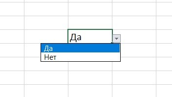
Next, the program will automatically create a drop-down menu in the appropriate cell. All information that the user has specified as items in the pop-up list. The rules for creating a list in several cells are similar to the previous ones, with the only exception that you must specify the information manually using a semicolon.

Creating a drop-down list using the OFFSET function

In addition to the classical method, it is possible to use the function ÀD .R.to generate dropdown menus.

Let’s open the sheet.

To use the function for the dropdown list, you need to do the following:

1. Select the cell of interest where you want to place the future list.
2. Open the “Data” tab and the “Data Validation” window in sequence.
   

   

3. Set “List”. This is done in the same way as the previous examples. Finally, the following formula is used: =OFFSET(A$2$;0;0;5). We enter it where the cells that will be used as an argument are specified.

Then the program will create a menu with a list of fruits.

The syntax for this is:

=OFFSET(reference,line_offset,column_offset,[height],[width])

We see that this function has 5 arguments. First, the first cell address to be offset is given. The next two arguments specify how many rows and columns to offset. Speaking of us, the Height argument is 5 because it represents the height of the list. 

Dropdown list in Excel with data substitution (+ using the OFFSET function)

In the given case ÀD .R. allowed to create a pop-up menu located in a fixed range. The disadvantage of this method is that after adding the item, you will have to edit the formula yourself.

To create a dynamic list with support for entering new information, you must:

1. Select the cell of interest.
2. Expand the “Data” tab and click on “Data Validation”.
3. In the window that opens, select the “List” item again and specify the following formula as the data source: =СМЕЩ(A$2$;0;0;СЧЕТЕСЛИ($A$2:$A$100;”<>”))
4. Tẹ Dara.

This contains a function COUNTIF, to immediately determine how many cells are filled (although it has a much larger number of uses, we just write it here for a specific purpose).

In order for the formula to function normally, it is necessary to trace whether there are empty cells on the path of the formula. They shouldn’t be.

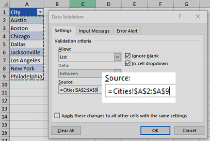
Dropdown list with data from another sheet or Excel file

The classic method does not work if you need to get information from another document or even a sheet contained in the same file. For this, the function is used TỌN, which allows you to enter in the correct format a link to a cell located in another sheet or in general – a file. You need to do the following:

1. Activate the cell where we place the list.
2. We open the window we already know. In the same place where we previously indicated sources for other ranges, a formula is indicated in the format =INDIRECT(“[List1.xlsx]Sheet1!$A$1:$A$9”). Naturally, instead of List1 and Sheet1, you can insert your book and sheet names, respectively. 

Attention! The file name is given in square brackets. In this case, Excel will not be able to use the file that is currently closed as a source of information.

It should also be noted that the file name itself makes sense only if the required document is located in the same folder as the one where the list will be inserted. If not, then you must specify the address of this document in full.

Ṣiṣẹda ti o gbẹkẹle Dropdowns

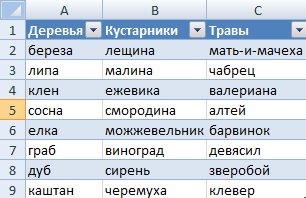
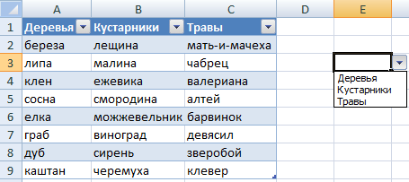
A dependent list is one whose contents are affected by the user’s choice in another list. Suppose we have a table open in front of us that contains three ranges, each of which has been given a name.

You need to follow these steps to generate lists whose result is affected by the option selected in another list.

1. Create 1st list with range names.
   

   

2. At the source entry point, the required indicators are highlighted one by one.
   

   

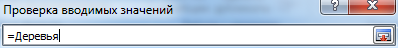
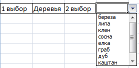
3. Create a 2nd list depending on the type of plant the person has chosen. Alternatively, if you specify trees in the first list, then the information in the second list will be “oak, hornbeam, chestnut” and beyond. It is necessary to write down the formula in the place of input of the data source =INDIRECT(E3). E3 – cell containing the name of the range 1.=INDIRECT(E3). E3 – cell with the name of the list 1.

Now everything is ready.

How to select multiple values ​​from a drop down list?

Sometimes it is not possible to give preference to only one value, so more than one must be selected. Then you need to add a macro to the page code. Using the key combination Alt + F11 opens the Visual Basic Editor. And the code is inserted there.

Iyipada Iṣẹ-iṣẹ Aladani Aladani (ByVal Target Bi Range)

    Lori Aṣiṣe aṣiṣe Itele

    If Not Intersect(Target, Range(«Е2:Е9»)) Is Nothing And Target.Cells.Count = 1 Then

        Application.EnableEvents = Eke

        If Len (Target.Offset (0, 1)) = 0 Then

            Target.Offset (0, 1) = Target

        miran

            Target.End (xlToRight) .Offset (0, 1) = Target

        Pari Ti

        Target.ClearContents

        Application.EnableEvents = Otitọ

    Pari Ti

Ipari ipari 

In order for the contents of the cells to be shown below, we insert the following code into the editor.

Iyipada Iṣẹ-iṣẹ Aladani Aladani (ByVal Target Bi Range)

    Lori Aṣiṣe aṣiṣe Itele

    If Not Intersect(Target, Range(«Н2:К2»)) Is Nothing And Target.Cells.Count = 1 Then

        Application.EnableEvents = Eke

        If Len (Target.Offset (1, 0)) = 0 Then

            Target.Offset (1, 0) = Target

        miran

            Target.End (xlDown) .Offset (1, 0) = Target

        Pari Ti

        Target.ClearContents

        Application.EnableEvents = Otitọ

    Pari Ti

Ipari ipari

And finally, this code is used to write in one cell.

Iyipada Iṣẹ-iṣẹ Aladani Aladani (ByVal Target Bi Range)

    Lori Aṣiṣe aṣiṣe Itele

    If Not Intersect(Target, Range(«C2:C5»)) Is Nothing And Target.Cells.Count = 1 Then

        Application.EnableEvents = Eke

        newVal = Target

        Application.Undo

        oldval = Target

        If Len (oldval) <> 0 And oldval <> newVal Then

            Target = Target & «,» & newVal

        miran

            Target = newVal

        Pari Ti

        If Len (newVal) = 0 Then Target.ClearContents

        Application.EnableEvents = Otitọ

    Pari Ti

Ipari ipari

Ranges are editable.

How to make a dropdown list with a search?

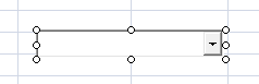
In this case, you must initially use a different type of list. The “Developer” tab opens, after which you need to click or tap (if the screen is touch) on the “Insert” – “ActiveX” element. It has a combo box. You will be prompted to draw this list, after which it will be added to the document.

Further, it is configured through properties, where a range is specified in the ListFillRange option. The cell where the user-defined value is displayed is configured using the LinkedCell option. Next, you just need to write down the first characters, as the program will automatically suggest possible values.

Dropdown list with automatic data substitution

There is also a function that the data is substituted automatically after they are added to the range. It’s easy to do this:

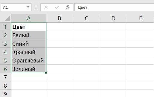
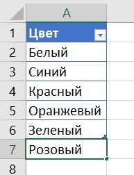
1. Create a set of cells for the future list. In our case, this is a set of colors. We select it.
   

   

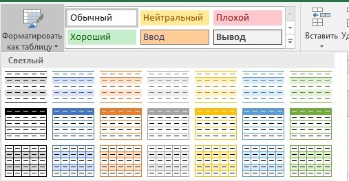
2. Next, it needs to be formatted as a table. You need to click the button of the same name and select the table style.
   

   

   

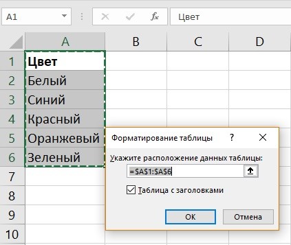
Next, you need to confirm this range by pressing the “OK” button.

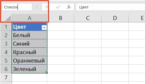
We select the resulting table and give it a name through the input field located on top of column A.

That’s it, there is a table, and it can be used as the basis for a drop-down list, for which you need:

1. Select the cell where the list is located.
2. Open the Data Validation dialog.
   

   

3. We set the data type to “List”, and as values ​​we give the name of the table through the = sign.
   

   

   

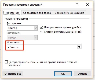
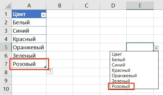
Everything, the cell is ready, and the names of the colors are shown in it, as we originally needed. Now you can add new positions simply by writing them in a cell located a little lower immediately after the last one.

This is the advantage of the table, that the range automatically increases when new data is added. Accordingly, this is the most convenient way to add a list.

How to copy drop down list?

To copy, it is enough to use the key combination Ctrl + C and Ctrl + V. So the drop-down list will be copied along with the formatting. To remove formatting, you need to use a special paste (in the context menu, this option appears after copying the list), where the “conditions on values” option is set.

Select all cells containing a drop down list

To accomplish this task, you must use the “Select a group of cells” function in the “Find and Select” group.

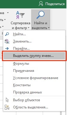
After that, a dialog box will open, where you should select the items “All” and “These same” in the “Data Validation” menu. The first item selects all lists, and the second selects only those that are similar to certain ones.